Introduction
In late 2016, I came across a TED talk titled Better Medicine Through Machine Learning. In it, Dr. Suchi Saria, an associate professor at Johns Hopkins University, presented how her team developed TREWS (Targeted Real-time Early Warning Score1) to help doctors assess a patient’s risk for septic shock2. Their revolutionary tool could tell which patients were at risk of experiencing septic shock at any given time.
TREWS was modeling when patients would fall sick! If it can do that for septic shock now, then imagine what else could be done for other ailments like cancers or heart attacks. That sounded incredible, and I had to learn more.
How does TREWS work? What kind of data do you need? What machine learning models are they using?
Craving these technical details, I delved into the TREWS white paper.
Maslow’s Hammer
TREWS is based on survival analysis, the statistical discipline of modeling the time to a specific event. That’s also why it’s sometimes called time-to-event analysis or failure analysis in engineering.
In the case of Dr. Saria and her team, they analyzed the time between a patient’s hospital admission and the onset of septic shock. But survival analysis can be applied to many domains, not just medicine. It can be used to predict time until divorce, customer attrition, incarceration, etc. It’s quite a general tool, but in the context of healthcare, it can make all the difference.
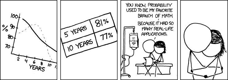
XKCD #881: Probability
What still eluded me was what survival analysis does differently than traditional techniques like linear regression3. Time is a continuous variable, so I wondered why tried and true methods were insufficient in predicting when an event would occur.
I suppose if all you have is a hammer, everything looks like a nail. While we can definitely use linear regression to predict time, survival analysis models time, not just predicts it. The nuance here is that survival analysis makes inferences about the survival of individuals and populations, in addition to forecasting illness. In other words, linear regression would only predict when septic shock would occur, and tell little of how patient populations succumb or survive over time.
In order to do these things, survival analysis incorporates information other than just survival time.4
Survival Data
Survival analysis primarily focuses on two variables:
- What is the survival time?
- Did the event in question occur?
The first question observes the exact duration of survival up to an event, compelling us to be explicit about when we start observing our patient, and when to stop.
The second question presents the idea that septic shock may not occur at all, so we have to take that into consideration when assessing survival time and making inferences.
These questions examine survival events, which are the boundaries for how long a patient survives. This will establish the foundation and common terminology prior to discussing modeling.
Survival Events
The birth event is the beginning, the starting point from which we begin to track the patient over time. It motivates us to observe the patient in the first place; in TREWS, the birth event is when the patient is first admitted to a hospital.
The death event marks the moment that a patient experiences the medical complication in question. This event answers the second question that we explored above. It could be when a patient dies, or in the case of TREWS, when a patient experiences septic shock.
Consequently, a patient survived if they don’t experience the death event, and they failed if they do.
For example, if we want to model the time until a computer crashes, the birth event could be the moment the computer was first booted up. The death event is the computer crash.
We can then restate our motivating questions in better terms:
- What is the time since the birth event?
- Did the death event occur?
While intuitive, this method of representing patient experiences now leads us to a new problem:
What if a patient never experiences a specific event? Can we still use the data if a patient doesn't experience septic shock, or experiences it before admission to a hospital?
“Censoring” Data
These scenarios occur fairly frequently, so it’s necessary to accommodate them in our dataset instead of leaving them out. We need information on both survivors and non-survivors to make our predictions as robust as possible. To that end, survival analysis uses censoring to describe when patients experience or don’t experience the death event.
Data is considered censored when knowledge of survival events is unavailable or not present. The following types of censoring specify how this can be the case.
Right Censoring
Patients are right-censored if they never experience the death event during observation. In TREWS, patients that never experience septic shock are right-censored, as it’s unclear if they will experience septic shock after they’re released from the hospital, or if they’re simply healthy.
This ambiguity in the patient’s health is why data is right-censored. Some research studies may report a “Lost to Follow Up”, which implies that a patient wasn’t tracked during a study, and those patients are usually right-censored as well.
Left Censoring
Samples are left-censored if they experience the death event before they were selected for observation. Restated, a patient may experience septic shock at home, before their admission to the hospital.
Left-censoring allows us to include failure cases like the one mentioned, but it also makes modeling survival time complicated because there’s no birth event to start the timer. That’s generally why this kind of censoring isn’t typically useful.
Interval Censoring
Samples are interval-censored if they experience the death event within an interval of time, so the exact time of the death event is unknown. For example, if a study tracks patients every 6 months, then a patient who experienced a death event would’ve experienced it anytime during a 6 month period.
Empowering Insights
These facets of survival data, events and censoring, are necessary to drive important insights about survival time and survival rates. Because this data is so rich, the application of traditional machine learning methods like linear regression and support vector machines leave much to be desired in this area.
Survival analysis is thus uniquely suited to solving the problems that TREWS grapples with by capitalizing on this extra information. It’s also part of the reason why TREWS works so well.
But this extra information is useless without a means to deconstruct, understand, and eventually model it. If we’re not using conventional approaches, then we need a different mathematical framework to help us capture the patterns inherent in survival data. This is where survival analysis really shines.
Survival Statistics
The Survivor Function
Survival analysis is driven partly by the survivor function, which calculates the probability of a sample surviving beyond a specified time. In other words, it examines how likely it is that septic shock hasn’t occurred yet.
In mathematical terms, the survivor function $S(t)$ provides the probability that a sample doesn’t experience the death event before a time $t$, assuming $t = 0$ is the birth event.
Let’s assume that $T$ is the random variable representing the time to the death event of a patient. The survivor function then measures the probability that the true survival time $T$ is greater than the time $t$ right at this moment. This can be written as follows:
$$S(t)=P(T>t)$$
For example, if we want to know the probability that a patient hasn’t experienced septic shock 3 hours after hospital admission, we simply calculate $S(3)$.
$$S(3)=P(T>3)$$
Given this, there are some theoretical conclusions we can draw about the survivor function. These should be familiar to anyone with a background in statistics and probability.
- $S(t)$ is a cumulative probability distribution.
- $S(t)$ is a continuous, smooth function.
- $S(t)$ is a non-increasing function.
- $S(0)=1$ because no sample experiences the death event at time $t=0$ (birth event).
- $S(\infty)=0$ because eventually, all samples experience the death event (or simply death).
In practice, however, there is no way for us to determine the survivor function $S(t)$ from data. We can instead try to estimate the survivor function, represented as $\hat{\text{S}}(t)$ (pronounced “S-hat of t”).
Estimated survivor functions are step-wise functions instead of continuous, smooth curves because they’re fitted to the data; as more data is available, the function will become smoother. In addition, $\hat{\text{S}}(t)$ may never equal $0$ because the death events may be right-censored.
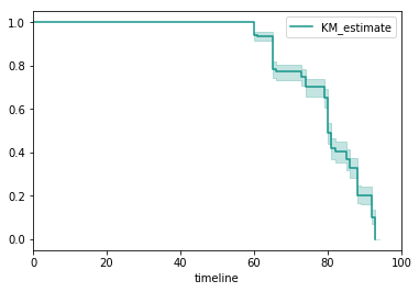
Plot of estimated survivor function over time with confidence intervals
The survivor function is not only a convenient representation, but also a powerful way to model survival rates. Using this mathematical tool we’re able to create a summary of overall patient survival, and this can inform physicians and patients how a malady generally progresses over time.
Unfortunately, there’s not much more we can learn from this information. We know that the probability of survival decreases over time, but the rate at which the death event occurs may not be so straightforward. For example, septic shock has periods of time when mortality rates spike, and then resolve.5
If I want to know which patients have the highest chance of experiencing septic shock in the next five minutes, or even the next five hours, I’m suddenly at a loss.
Will a doctor know who to treat for septic shock right away, if they only know the probability that any patient would survive the next day?
We need a way to model the risk that the death event will occur at any time, by tracking the rate at which death events occur.
The Hazard Function
The hazard function is the counterpart to the survivor function, and is the other workhorse of survival analysis. Unlike the survivor function, which is just a measure of probability, the hazard function is a ratio of probability and time. To help us understand exactly what the hazard function does, we’ll first reexamine why we need it and what it represents.
Recall that the survivor function can be used to make population-level inferences about a patient: the probability that a patient survives past a given time $t$. But all patients are not the same, and one may be declining in health at a faster rate than another. More importantly, all ailments are not the same, and some have periodic mortality rates, in which the probability of experiencing the death event rises and falls repeatedly.
To model these facets of survival, we turn to the hazard function. The formula for the hazard function $ h(t) $ is as follows:
$$ h(t) = \lim_{\Delta t \to 0} \frac{P(t \leq T \leq t + \Delta t | T \geq t)}{\Delta t} $$
In mathematical terms, the hazard function measures the instantaneous probability that a sample will experience the death event at time $t$, assuming the sample has survived to time $t$. We assume that the patient survives until that point, and given that assumption, calculate the conditional probability that the patient will experience septic shock. The hazard function is a measure of probability over a time interval, which is why it’s a rate and not a probability.
There’s clearly a lot going on here, so let’s break it down piece by piece. We’ll first touch on the numerator, and then use the analogy of speed to examine the limit and denominator. Taken altogether, we’ll be able to interpret the hazard function.
The Time Frame of Death
$$P(t \leq T \leq t + \Delta t | T \geq t)$$
The numerator describes the conditional probability that the time of the death event $T$ falls in the time interval $ [t, t + \Delta t] $, assuming that the patient at least survives to the given time $t$.
When the size of the interval $\Delta{t}$ is large and approaching $\infty$, the conditional probability will approach $1$; the larger the interval, the more likely it is that the death event will occur in it. Conversely, the smaller the interval, the lower the probability.
By itself, this expression can provide the conditional probability that the death event will occur in the next second, the next hour, or the next day, depending on the size of the time interval.
But what happens if we try to shrink the time interval to an infinitesimally small size?
To help us answer this question, we refer to a very familiar ratio: speed.
A Parallel to Instantaneous Speed
Let’s digress a little from survival analysis. Consider the following situation:
Suppose I have to drive from San Francisco to Los Angeles for a conference. My insurance company thinks I’ve been driving too fast lately, so just to prove them wrong I decide to record my speed on this trip.
Once I reach LA, I review my numbers and find that I drove 383 miles for 6 hours and 15 minutes.
Average speed is calculated through the following formulas: $ \frac{x}{t} $ or $ \frac{\textit{distance between SF and LA}}{\textit{how long the drive to LA took}} $. That means that my average speed would be $ \frac{383}{6.25} $ or $ 61.28 $ mph for this leg of the journey, which is below the rural highway speed limit of 70 mph.
On my way back to SF, however, I glance at my speedometer and notice that I’m driving at 78 mph. This is the instantaneous speed, or the speed at the instant that I looked at my speedometer.
Instantaneous speed is determined through the following formulas: $ \lim_{\Delta{t} \to 0} \frac{\Delta{x}}{\Delta{t}} $ or $ \lim_{\textit{change in time} \to 0} \frac{\textit{change in position}}{\textit{change in time}} $. This formulation describes how an “instant” is actually a really small time interval, so the change in time is infinitesimally small and really close in value to $ 0 $. In comparison, when we calculate average speed, the time interval is the total time of our drive.
Interestingly, when I reach SF, I find that my average speed for the return leg is the same as my outbound leg: 61.28 mph. At first, I’m convinced that I drive safely, contrary to my insurer’s claims. But then I remember my speedometer reading of 78 mph.
It doesn’t matter what my average speed for a trip is, if at any instant I’m driving over the speed limit! So while the average speed is useful if I want a summary of my speed during my drive, instantaneous speed is more relevant when I’m concerned about things like speed limits. This resembles our dilemma with the survivor function and the consequent need for the hazard function.
More importantly, the instantaneous speed is also conveying the potential number of miles I can travel in the next hour. In other words, if my speed at a moment is 78 mph, then I can potentially drive 78 miles in the next hour if I maintain that speed. But that’s not necessarily the outcome, given that my average speed was much lower.
The hazard function is based on this abstraction, but instead of speed we consider the probability of observing the death event. Instantaneous speed measures the potential miles per hour I can drive at a given moment. The hazard function measures the potential that the death event will occur at a given moment.
Still, speed as a ratio is not a perfect analogy to the hazard function. Recall the expression again:
$$ h(t) = \lim_{\Delta t \to 0} \frac{P(t \leq T \leq t + \Delta t | T \geq t)}{\Delta t} $$
Notice that while speed ($ \frac{\Delta{x}}{\Delta{t}} $) is a first derivative of position (the $\Delta$ on the numerator and denominator), the hazard function is not a derivative; the numerator is simply a probability, not a change in probability. Although speed is an apt analogy to explain instantaneous potential, it alone isn’t sufficient to explain the nature of the numerator.
Putting It All Together
In essence, the numerator is the conditional probability that the death event occurs in that interval. The denominator is the size of the interval, $ \Delta t $.
As with instantaneous speed, we take the limit of this expression as the time interval approaches 0 in size to calculate the instantaneous probability, or hazard rate at that instant. As the interval becomes very small, we can estimate the value of the expression at a given time $ t $, for any time step.
For example, if we want to know the hazard of a patient experiencing septic shock 3 hours after hospital admission, we determine the conditional probability of failure over an interval.
$$ h(t) = \lim_{\Delta t \to 0} \frac{P(3 \leq T \leq 3 + \Delta t | T \geq 3)}{\Delta t} $$
Assuming that the time of the death event $ T $ is greater than or equal to 3 hours, we can then calculate the probability that the death event occurs within a small interval between $ 3 $ and $ 3 + \Delta t $. This interval becomes smaller as $ \Delta t $ approaches 0. We find the hazard rate by scaling the probability by said interval size, $ \Delta t $.
The hazard function is then the rate at which the conditional probability of the death event occurs at a given instant. For this reason, the hazard function is also sometimes referred to as the conditional failure rate.
It may be easier to think of the hazard rate as the perceived risk that a patient will experience the death event at a given moment. So the higher the hazard rate, the higher the risk. The greater the hazard, the greater the risk of septic shock.
It’s important then to realize the following.
- $ h(t) $ can produce a value that is greater than 1, since it’s not a probability and is scaled by $\Delta t$ .
- $ h(t) $ will differ depending on the units of time used, as the units affect the size of the window that the death event occurs in.
- $ h(t) $ has no upper bound.
- $ h(t) $ is always greater than or equal to 0.
As mentioned, the hazard function traditionally has a lower bound of 0, even though it has no upper bound as per the formula. More recently, however, novel modeling techniques tend to relax this principle and calculate negative rates, though that’s out of the scope of this article.
However, the most important property of the hazard function is that it’s a relative measure. In other words, the result of one hazard expression only has meaning when compared to another result. Thus, we can compare two patients’ hazards, and determine which may be in a more “dangerous” condition. This is the essential utility of the hazard function.
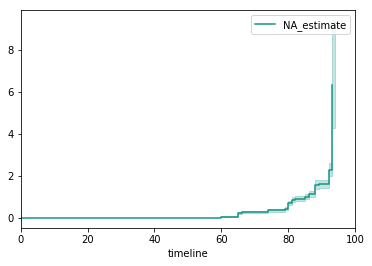
Plot of estimated hazard function over time with confidence intervals
Naturally, the estimated hazard function $ \hat{h}(t) $ is also modeled as a step-wise function.
Equipped with the survivor and hazard functions, we’re able to understand survival data in a meaningful way. By revealing how patients survive over time and the rate at which death events are observed, we can now make clinical decisions based on our mathematical model. This is empowering to not only a physician, but also to the patients who want to better understand their health.
Two Sides to the Same Story
You may have realized as I did that the survivor and hazard functions aren’t independent of each other. While the survivor function measures the probability of not seeing the death event, the hazard function assesses the potential of the death event. The survivor function models a cumulative distribution over time, and the hazard function monitors instantaneous events.
Even more interesting, we can derive each function from the other. They’re generalized as the following:
$$ S(t) = exp \bigg(- \int_0^{t} h(u) du \bigg) $$
$$ h(t) = - \frac{dS(t)}{S(t) dt} $$
There are many methods that model survivor and hazard curves, and each makes their own assumptions as to which function to model first. Typically, it’s the hazard function. Regardless of the approach, both the survivor and hazard functions are powerful ways to reason about survival data and help make clinical decisions.
Final Thoughts
In some shape or form, survival analysis exists in all analytical disciplines, whether it’s business analytics, epidemiology, manufacturing, sociology, etc. And what makes it so compelling is that we can use it in any way we imagine, from analyzing network outages and engine failure to understanding homelessness and divorce. I chanced upon this subject because I watched a YouTube video, but its utility shapes the way I view many statistical and clinical problems.
Survival analysis gives us the tools to model the time to an event, and not just forecast it. The unique nature of survival events and censoring enables key insight into how and when patients succumb to illnesses or survive. Mathematical modeling of this survival data through survivor and hazard functions provides the information to make clinical decisions and even predict when patients will experience the death event without intervention.
These terms and concepts give us the foundation to tackle more interesting problems, like how to fit survivor and hazard curves and predict death events. In a future article, we’ll examine these methods and the Cox-PH model, which is the core of the TREWS system.
Footnotes
[2] a life-threatening severe form of sepsis that usually results from the presence of bacteria and their toxins in the bloodstream and is characterized especially by persistent hypotension with reduced blood flow to organs and tissues and often organ dysfunction — Merriam-Webster
[3] Linear Regression, Wikipedia
[4] "Unlike ordinary regression models, survival methods correctly incorporate information from both censored and uncensored observations in estimating important model parameters. The dependent variable in survival analysis is composed of two parts: one is the time to event and the other is the event status, which records if the event of interest occurred or not. One can then estimate two functions that are dependent on time, the survival and hazard functions." excerpt from "What is Survival Analysis?"